Recreate a NPR graphic in ggplot

This is an attempt to continue the work that @hrbrmstr did at Coloring (and Drawing) Outside the Lines in ggplot.

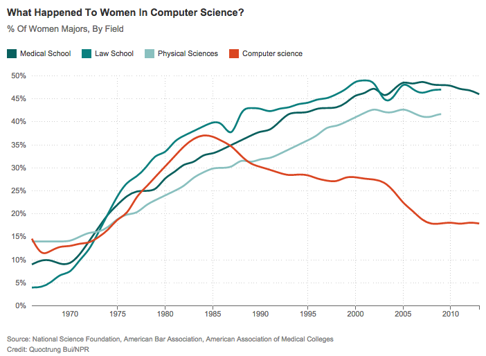
It all started with a tweet asking for a way to replicate this graphic in ggplot.

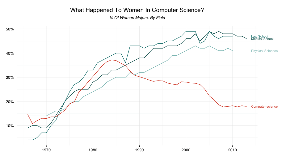
This is the plot that @hrbrmstr created (in ggplot) at the end of his post.

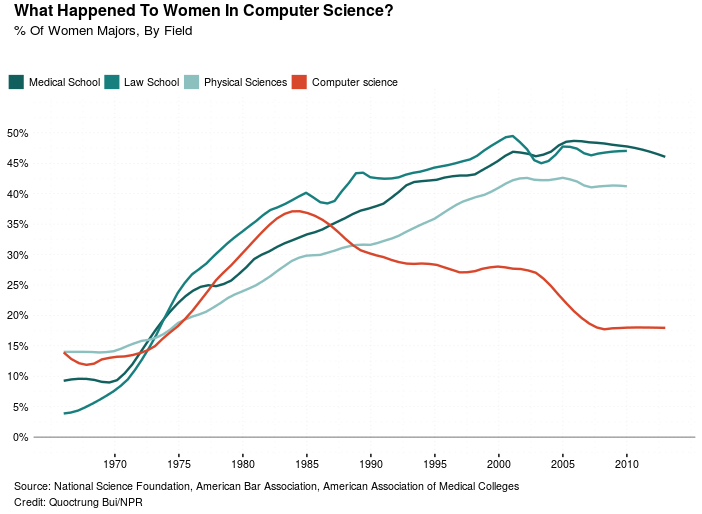
I took his code, and tweaked it to get the ggplot version to be as similar as possible to the original plot. Here is what I achieved:

Code (some of it is taken from the @hrbrmstr’s blog post):

(Code is also available at github.com/sainathadapa)

library(ggplot2)
library(dplyr)
library(tidyr)
library(stringr)
library(scales)
library(gridExtra)
library(grid)
library(Cairo)
library(gtable)

# use the NPR story data file ---------------------------------------------
# and be kind to NPR's bandwidth budget
url <- "http://apps.npr.org/dailygraphics/graphics/women-cs/data.csv"
fil <- "gender.csv"
if (!file.exists(fil)) download.file(url, fil)

gender <- read.csv(fil, stringsAsFactors=FALSE)

# take a look at the CSV structure ----------------------------------------

glimpse(gender)

tail(gender)

# via http://apps.npr.org/dailygraphics/graphics/women-cs/js/graphic.js
# there are 'tk' values in the data set that should be ignored so
# replace them with NA by ensuring all columns are numeric.
# also the color values came from that javascript file, too.

gender <- mutate_each(gender, funs(as.numeric))

# make better column labels for display ----------------------------------

colnames(gender) <- str_replace(colnames(gender), "\\.", " ")

gender_long <- mutate(gather(gender, area, value, -date),
                      area=factor(area, levels=colnames(gender)[2:5],
                                  ordered=TRUE))

gender_colors <- c('#11605E', '#17807E', '#8BC0BF','#D8472B')
names(gender_colors) <- colnames(gender)[2:5]

# ggplot ------------------------------------------------------------------

gg <- ggplot(gender_long)

# Using LOESS smoothing for the lines
gg <- gg + geom_smooth(aes(x = date, y = value, group = area, color = area),
                           se = F, method = "loess", span = 0.15, size = 0.85) +
           geom_hline(yintercept = 0, size = 0.2) +
           scale_color_manual(name = "", values = gender_colors) +
           scale_y_continuous(label = percent,
                              breaks = seq(from = 0,to = 0.5,by = 0.05)) +
           scale_x_continuous(breaks = seq(from = 1970, to = 2010, by = 5)) +
           coord_cartesian(xlim = c(1966, 2013), ylim = c(0, 0.55)) +
           labs(x = NULL, y = NULL, title = NULL)

# Theme settings
gg <- gg + theme_bw(base_family = "Helvetica", base_size = 10)
gg <- gg + theme(axis.ticks.y          = element_blank(),
                 panel.border          = element_blank(),
                 legend.key            = element_blank(),
                 legend.justification  = 'left',
                 legend.position       = c(-0.075,1.01),
                 legend.direction      = 'horizontal'),
                 legend.key.height     = unit(0.1, 'cm'),
                 legend.key.width      = unit(0.1, 'cm'),
                 panel.grid            = element_line(linetype = 'dotted',
                                                      size     = 1,
                                                      color    = 'black'))
gg <- gg + guides(colour = guide_legend(override.aes = list(size = 5)))


# Needed to use viewports to align and size the text properly
vplayout <- function(x, y) viewport(layout.pos.row = x, layout.pos.col = y)

gg1 <- textGrob(expression(bold("What Happened To Women In Computer Science?")),
                vp    = vplayout(1,1),
                x     = unit(0.02, "npc"),
                y     = unit(0.5, "npc"),
                hjust = 0,
                vjust = 0,
                gp    = gpar(fontsize = 12, face = "bold", col = "black"))

gg2 <- textGrob("% Of Women Majors, By Field",
                vp    = vplayout(2,1),
                hjust = 0,
                vjust = -0.5,
                x     = unit(0.02, "npc"),
                y     = unit(1, "npc"),
                just  = "left",
                gp    = gpar(fontsize = 10,col = "black"))
gg3 <- gg

gg4 <- textGrob("Source: National Science Foundation, American Bar Association, American Association of Medical Colleges",
                x     = unit(0.02, "npc"),
                y     = unit(0, "npc"),
                hjust = 0,
                vjust = -0.5,
                vp    = vplayout(15,1),
                gp    = gpar(fontsize = 8, col = "black"))

gg5 <- textGrob("Credit: Quoctrung Bui/NPR",
                x     = unit(0.02, "npc"),
                y     = unit(0, "npc"),
                hjust = 0,
                vjust = -1,
                vp    = vplayout(16,1),
                gp    = gpar(fontsize = 8, col = "black"))

layout_matrix <- matrix(c(1,1, 2,2, rep(3, times = 20), 4, 5),ncol = 1)

# arrangeGrob (as the name says) to arrange the all the different elements
ggf <- arrangeGrob(gg1, gg2, gg3, gg4, gg5, layout_matrix = layout_matrix)

grid.draw(ggf)